Graph
A linear graph or simply a graph , consists of a set of objects, called vertices, and another set called edges such that each edge, , is identified with unordered pair of vertices.
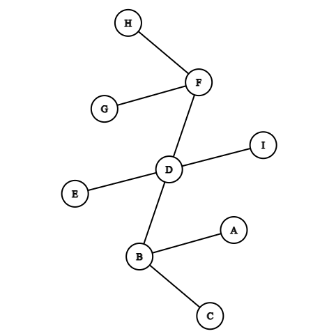
Following is an example of a simple graph:
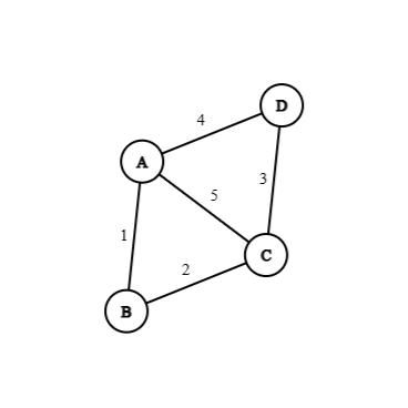
In the above example, the vertices set is: , and the edges set is:
Some Terms in Graph Theory
Following are some terms widely used in graph theory:
Self loop
An edge having the same vertex as both its end vertices is called a self loop.
Following is an example:
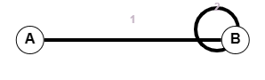
In the above example, edge 1 is a normal edge and edge 2 is a self loop with the same end vertices.
Parallel edges
If more than one edge is associated with a given pair og vertices, such edges are referred to as parallel edges.
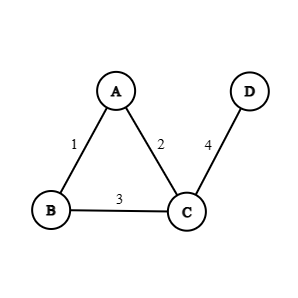
Given below is an example of a graph showing parallel edges:
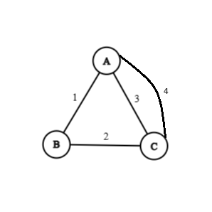
In the above example, edges 3 and 4 are examples of parallel edges.
Question: Discuss the gamous Koinsberg bridge problem and give a solution OR Discuss one real life applications of graph theory.
Finite and infinite graph
If in a graph the number of vertices and edges are finite then it is called a finite graph otherwise it is called an infinite graph.
| Type | Graph |
|---|---|
| Finite |  |
| Infinite |  |
Incidence
When a vertex is an end vertex of same edge , then and are said to be incident with each other.
In the following example, 3 is incident on B and C.
Adjacency
Two non-parallel edges are said to be adjacent if they are incident on a common vertex.
In the above example, 3&5 are non-adjacent due to a parallel edge between them. Other than that, all other edge pairs are adjacent to each other.
Degree of a vertex
The no. of edges incident on a vertex with self loop counted twice is called the degree of a vertex.
In the above example, following are the degrees:
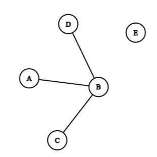
Isolated vertex
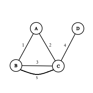
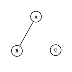
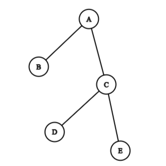
A vertex having no incident edge is called an isolated vertex. In the following example, C is an isolated vertex.
Pendant vertex
A vertex of degree 1 is called a pendant vertex or end vertex.
In the above example D is a pendant vertex.
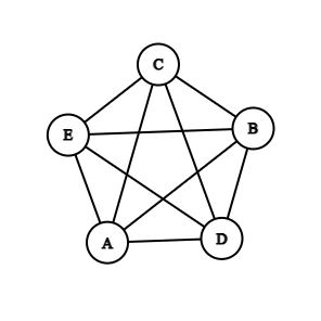
Regular graph
A graph in which all the vertices are of equal degree is called a regular graph. Following is an example of a regular graph:
Theorem 1
The number of vertices of odd degree in a graph is always even.
Let us consider vertices with odd degree and even degree seperately. Then, the total number of degrees in a graph can be expressed as follows:
We know, the total degree of a graph can be obtained by the number of edges (). Therefore equation can be written as:
Where, is the number of edges.
The first expression on the right hand side is even, (being the sum of even numbers). The left hand side is also the sum of even degrees, which is also even. Thus equation can be expressed as follows:
The subtraction of one even number from another even number results in an even number. Therefore the theorem that, the number of vertices of odd degree in a graph is always even, holds true.
Isomorphism
Two graphs and are said to be isomorphic if there is one-to-one correspondence between their vertices and their edges such that incidence relationship is maintained.
Thus for two isomorphic graph, it must have:
- Same number of vertices
- Same number of edges
- An equal number of vertices with a given degree
In the following examples, and are isomorphic graphs:
| Label | Graph |
|---|---|
 | |
 |
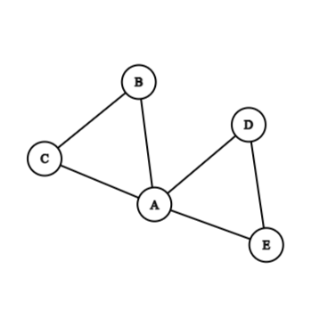
Example 1: "The criteria for isomorphism in the definition is insufficient." Justify this with an example.
Considering two graphs:
Graph having vertices set, be named , and be named .
According to the formal definition, both and are isomorphic because:
- They have equal number of vertices
- They have equal number of edges
- They have equal number of vertices with a given degree
The vertex in must correspond to the vertex in , as both their degree is 3. is associated with two pendant vertex whereas is associated with one pendant vertex, thus and are not really isomorphic.
Sub-graph
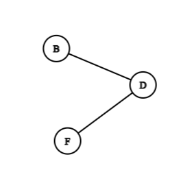
A graph is said to be a subgraph of a graph , if all the vertices and all the edges of are in and each edge of has the same end vertex in .
For example, in the following, is a subgraph of :
| Label | Graph |
|---|---|
| |
| (sub-graph) | 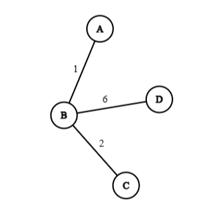 |
Characteristics of sub-graph
- Every graph is its own sub-graph
- A sub-graph of a sub-graph of is also a sub-graph of
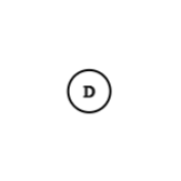
- A single vertex of is also a sub-graph of
- A single edge of along with its end vertices is also a sub-graph of .
Operations on Graphs
Union
The union of two graphs, , and is anothe graph, , whose vertex set , and edge set is .
Following is the example of graphical union:
| Label | Graph |
|---|---|
| |
 | |
 |
Intersection
The intersection of two graphs and , is another graph , whose vertex set, , and edge set is, .
Following is the example of graphical intersection:
| Label | Graph |
|---|---|
| |
| |
 |
Ring sum
The ring sum of two graphs , and , is another graph , written as whose vertex set , and edge set having those edges that are either in or in but not in both.
| Label | Graph |
|---|---|
| |
| |
 |
Fusion
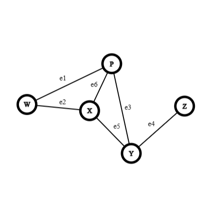
A pair of vertices in a graph are said to be fused if the two vertices are replaced by a single new vertex such that every edge that was incident on either or or both are now incident on the new vertex.
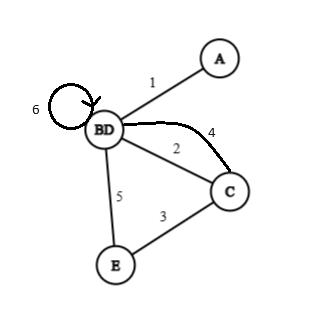
Considering the following graph:
In the above graph when and are fused, we get the following, where edge 6 forms a self-loop and edge 2 and 4 are parallel.
Decomposition
A graph is said to have been decomposed into two sub-graphs and such that:
Example:
| Label | Graph |
|---|---|
| |
| Decomposed part |  |
| Final graph |  |
Matrix Representation of a Graph
Incidence matrix
Let be a graph, with vertices, edges, and no self loops, then incidence matrix is an matrix, , whose rows corresponds to vertices, and columns correspond to edges.
The following holds true:
- , if edge is incident on vertex
- , otherwise
Considering the following example:
Incidence matrix of the above graph:
Characteristics
- The number of 1s in a row gives the degree of the corresponding matrix.
- Every edge is on exactly two vertices, hence every column has exactly two 1s.
- A row with all 0s corresponds to an isolated vertex.
- A column of single 1s would represent a self loop.
- Two identical columns represent parallel edges.
Adjacency matrix
The adjacency matrix of a graph with vertices and no parallel edges is an matrix , whose elements:
- , if there is an edge between and vertex
- , otherwise
Considering the following example:
Adjacency matrix of the above graph is:
Characteristics
- The diagonal elements are zero if there are no self loop.
- The number of 1s in a row or column gives the degree of that vertex.
- There are no provision for parallel edges because that information cannot be stored in the matrix.
- A row or column of all 0s correspond to an isolated matrix.
- A matrix of all zeros represent a null graph.
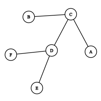
Example 2: Draw a graph corresponding to the following matrix:
The graph represented by the above matrix is:
Circuit matrix
Let the number of different circuits in a graph be and the number of edges in be , then the circuit matrix is a matrix whose elements are:
- , if the circuit includes edge
- , otherwise
Considering the following example of a graph:
The above represented in circuit matrix will be:
Characteristics
- The number of 1s in a row denotes the number of edges participating in the circuit.
- A column of all zeros denotes an edge which is not part of any circuit.
- A single 1 in a row denotes a self loop.
- Two graphs , and are isomorphic if they have the same circuit matrix.
- A column of all 1s denotes an edge which is a part of all circuits.
Path matrix
A path matrix for a specific pair of vertices say , and is written as , where the number of rows denotes the different available paths between and , and columns represent the edges.
- , if edge lies in path
- , otherwise
The same vertex cannot be travelled twice.
Considering the example for a following graph:
The path matrix between and is:
Characteistics
- A column of all zeros, represents an edge which is not a part of any edge of the paths.
- A column of all 1s represent an edge which is a part of all the paths.
- The number of 1s in a row give the path length.
- It only works for two given vertices.
- Path matrix cannot be attained if both vertices source and destination are the same.
Sub Sections of a Graph
Following are the different sections in which a graph can be sub-divided into:
Walk
A walk is defined as a finite alternating sequence of vertices and edges beginning and ending with vertices such that each edge is incident with vertices preceeding and following it. No edge appears more than once in a walk.
A single vertex cannot be a part of a walk.
Open and closed walk
If it is possible for a walk to begin and end at the same vertex such a walk is called a closed walk. A walk that is not closed is called an open walk.
In the above example, transversing AECDB is an open walk., while AEBDCA is a closed walk.
Another example of walk is, AEDCE
Path
An open walk in which no vertex appears more than once is called a path. The number of edges in the path is called length of the path.
In the above example, AECDB is a path with a path length of 4.
All paths are a walk, but all walks are not a path.
A path has to be an open walk.
Circuit
A closed walk in which no vertex except the initial and final appears more than once is called a circuit.
In the above example, AECBDA is a circuit.
A self loop is the smallest circuit.
A circuit has to be a closed loop.
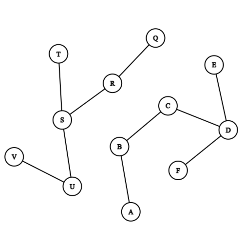
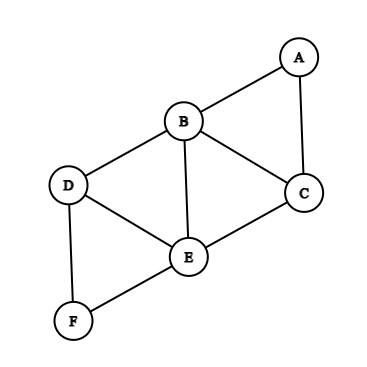
Connected and disconnected graph
A graph is said to be connected if there is atleast one path between every pair of vertices otherwise it is disconnected.
The above graph is a connected graph as all vertices are joined by atleast one edge.
Theorem 2
A simple graph with vertices and components, can have atmost edges, where, is:
Proof
Let the number of vertices in each of the components be . Thus we have:
We can derive:
Squaring both sides we get:
After removing the non-negative cross term, we get:
The maximum number of edges in the component is . Therefore, the maximum number of edges in the graph is equal to:
From eq. we can write:
Thus, taking the maximum value from above, we can state a simple graph with vertices and components can have at most, elements as stated below:
Hence the theorem.
Forms of Graph
There are two most popular forms of graphs: Euler Graph, and Hamiltonian Circuit.
Euler Graph
If some closed walk in a graph contains all the edges of the graph then the walk is called an Euler Line, and the graph is called an Euler Graph.
Each vertex should have even degree to allow entry as well as exit points.
The above is an example of an Euler Graph, transversing ACBADEA.
Hamiltonian Circuit
A Hamiltonian Circuit is a connected graph and is defined as a closed walk that traverses every vertex exactly once except of course the starting vertex at which the walk also terminates.
It is not necessary to travel all edges in Hamiltonian Circuit.
There are two Hamiltonian Circuits in the above graph: ACBA and ADEA.
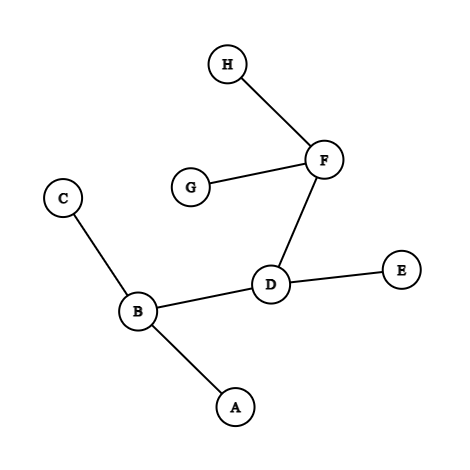
Tree
A tree is a connected graph without circuit. In the following example: , and are trees:
| Label | Graph |
|---|---|
 | |
 |
Theorem 3
A tree with vertices, has edges.
Proof
The theorem will be proved by induction on the number of vertices.
| No. of vertices | No. of edges |
|---|---|
Let us assume that the theorem holds true for vertices, with the maximum number of edges amounting to . If we can prove that the theorem holds true for then it holds true for all values of .
Let us consider a tree with vertices. In , let be an edge that connects two vertices and . Division of will disconnect the tree into two subtrees, (with vertices), and (with vertices). There cannot be any other path between and , otherwise it will form an circuit.
Both and has less than or equal to vertices hence the theorem should hold true for for both and .
We know:
Subtree has edges, and subtree has edges. Therefore, the total number of edges is the sum of edges of and from the edge where the tree was broken into two subtrees. Therefore total edges in tree , is:
Therefore, the maximum number of edges in a tree, with vertices is .
Definitions Used to Characterize Graphs
Distance
In a connected graph , the distance between two of its vertices and is the length of the shortest path between and , i.e., the number of edges in the shortest path between and . Example:
In the above graph, the distance between , and is: .
Metric Function
A function , is called a metric function, if it satisfies the following three conditions:
- Non-negativity: , and
- Symmetry:
- Triangular Inequality: , for any
Example 3: Show with an example that distance in a graph is a metric function.
In order to show that distance is a metric function, the graph must exhibit: non-negativity, symmetry and triangular inequality.
Considering the following example:
-
Non-negativity: The number of edges in a path between two vertices can never be negative but can be zero if source and destination vertices are same. Example: , and
-
Symmetry:
-
Triangular inequality: We have: . Therefore the following holds true:
Which holds true, hence distance exhibits triangular inequality.
Eccentricity
The eccentricity of a vertex in a graph is the distance from to , the farthest distance from in , as shown by the following equation:
In the above example, the eccentricity are as follows:
Eccentricities are to be calculated for edges not shared with pendant vertices.
Center
A vertex with minimum eccentricity in a graph , is called its center.
In the above example the vertex with the lowest eccentricity is . Therefore, is the center vertex.
Theorem 4
Every tree has either one or two center.
Considering the following graph:
Proof
The maximum distance from a given vertex to any vertex can only occur if is a pendant vertex. With this observation we delete all the pendent vertex from to obtain
The vertices in have one less eccentricity than . Thus the center or centers of are still center or centers in .
We continue this process of deleting pendent vertices to obtain , until we are left with a tree with vengle vertex (one center), or a tree with two vertices and an edge, (two center), hence the theorem.
After two successful removal of pendant vertex, we get, , and as:
| Label | Tree |
|---|---|
 | |
 |
Radius
The eccentricity of the center is called the radius of the tree. Following is the example of a graph:
In the above graph, and are the centers, and their eccentricity are , therefore, the radius is 2.
Diameter
The diameter of a tree is the length of the longest path in , i.e., the path with maximum eccentricity.
In the above diagram, the length of the longest path is 3, so diameter of the tree is 3.
It is not necessary that the diameter of a tree is always twice of its radius.
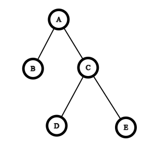
Rooted tree
A tree in which one vertex is distinguishable from all the other vertices is called a rooted tree.
In the above diagram, vertex is a root vertex.
Binary rooted tree
A special class of rooted tree called binary rooted tree in which exactly one vertex is of degree two, and the remaining are of degree one or three.
The above is a binary rooted tree.
Example 4: If there are total vertices in a binary rooted tree, then how many vertices are of degree ?
We know:
Where, is the number of pendant vertices, and is the total number of vertices.
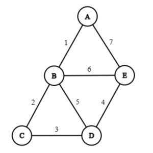
Spanning tree
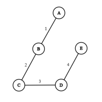
A tree is said to be spanning tree of a connected graph , if is a subgraph of and contains all vertices of . Spanning tree is also called a skeleton.
Following is an example of a graph and its spanning tree :
| Label | Diagram |
|---|---|
 | |
 |
Distance between spanning tree:
The distance between two spanning trees and of a graph is defined as the number of edges present in but not in . It is written as .
Considering the following example
| Label | Diagram |
|---|---|
 | |
 | |
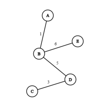 |
In the above graph and trees:
Example 5: Show with an example that distance between spanning trees is a metric function.
Considering the example used in the above pictures:
Non-negativity:
The number of edges present in one tree but not in the other tree cannot be a negative number, but a minimum of as in .
Symmetry:
As in the above example, the number of edges not found in one tree of a graph, but found in the other tree of the same graph, in order to determine the distance, and vice versa. Therefore, the distance in two trees will be the same with respect to both the trees, hence they are symmetric.
Triangular inequality:
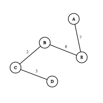
Considering another tree of the graph as:
For triangular inequality the following condition must hold true:
Since the above condition holds true, therefore triangular inequality satisfies.
Minimal Spanning Tree
A spanning tree with the smallest weight in a weighted graph is called a shortest spanning tree or minimal spanning tree.
There are two ways to find minimal spanning tree:
- Prim's algorithm
- Kruskal's algorithm
Prim's algorithm
This algorithm is used to find the shortest spanning tree of a graph with vertices.
Steps
-
Draw isolated vertices and label them, .
-
Tabulate the given weights of the edges of in an matrix. (set the diagonals as empty and non-existing direct edges as infinity ()).
-
Start from vertex and connect to its nearest neighbour (i.e., choose the smallest entry in root).
-
Repeat Steps (5,6), untill edges have been selected.
-
Consider the previous selected row(s) and the currently selected row and choose the next smallest weight in the selected rows.
-
While considering the smallest weight, neglect those edges who have been already selected or those edges which forms a circuit.
-
Exit when all rows have been selected.
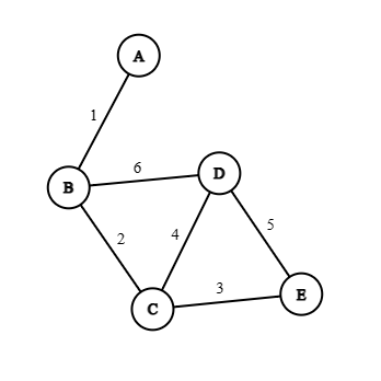
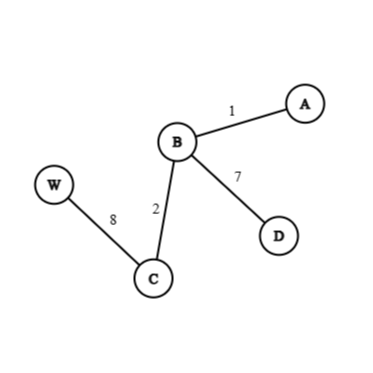
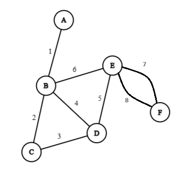
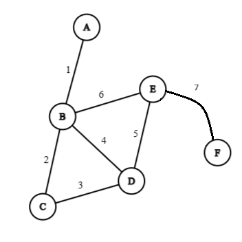
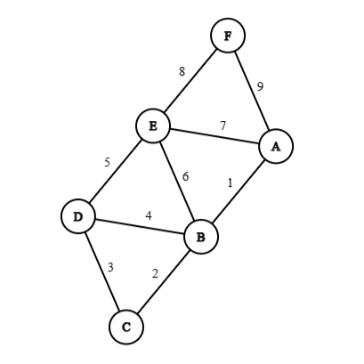
Example 6: Find minimal spanning tree using Prim's algorithm for the following graph, where the edge labels denote their weights.
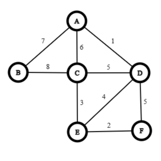
Matrix tabulation
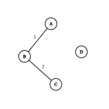
From the above matrix we can find out that, the minimum spanning tree is:
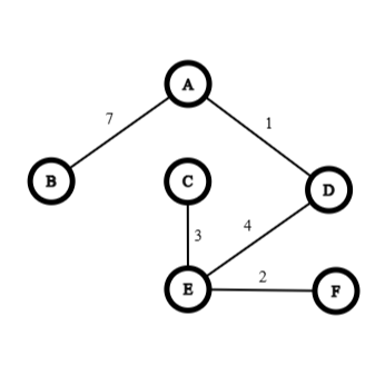
Minimum spanning weight, :
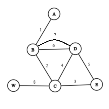
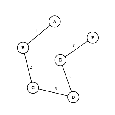
Example 7: Find minimal spanning tree using Prim's algorithm for the following graph, where edge label denote the weight.
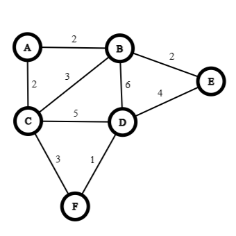
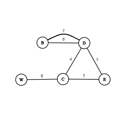
From the above matrix we can find out that the minimum spanning tree is:
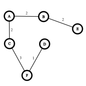
Minimal spanning weight, is: